
Main Task : CNN, Create Model, Pretrained Model(VGG16), Fine tuning
Main library : Tensorflow_datasets, Tensorflow.keras
보노보노는 강아지였나?
Dataset
데이터셋은 텐서플로우에서 제공하는 데이터셋을 사용합니다
23262장의 이미지를 가지고 있습니다
고양이 대 개 | TensorFlow Datasets
도움말 Kaggle에 TensorFlow과 그레이트 배리어 리프 (Great Barrier Reef)를 보호하기 도전에 참여 이 페이지는 Cloud Translation API를 통해 번역되었습니다. Switch to English 고양이 대 개 고양이와 개 이미지의
www.tensorflow.org
23262장 중에 80퍼는 train, 10퍼는 valid, 10퍼는 test 셋으로 분리합니다
import tensorflow as tf
import tensorflow_datasets as tfds
(raw_train, raw_validation, raw_test), metadata = tfds.load(
    'cats_vs_dogs',
    split=['train[:80%]','train[80%:90%]','train[90%:]'],
    with_info=True,
    as_supervised=True
)
# data download
Data feature
이미지의 shape가 None으로 나오는데 이는 각 이미지들의 사이즈가 달라서
규정할 수 없기 때문입니다
print(raw_train, raw_validation, raw_test, sep='\n')

#<PrefetchDataset shapes: ((None, None, 3), ()), types: (tf.uint8, tf.int64)>
<PrefetchDataset shapes: ((None, None, 3), ()), types: (tf.uint8, tf.int64)>
<PrefetchDataset shapes: ((None, None, 3), ()), types: (tf.uint8, tf.int64)>
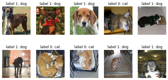
개와 고양이 누가 귀여운가의 대결로 착각 할 뻔 했네요
import matplotlib.pyplot as plt
plt.figure(figsize=(10,5))

get_label_name = metadata.features['label'].int2str
# take() create new dataset instance as much as parameter
for idx, (image, label) in enumerate(raw_train.take(10)):
    plt.subplot(2, 5, idx+1)
    plt.imshow(image)
    plt.title(f'label {label}: {get_label_name(label)}')
    plt.axis('off')
Data Preprocess
Image resize
각각의 이미지 크기가 다르므로 이미지 크기를 조정합니다
예제의 데이터를 사용했기 때문에 생략되었지만
각 데이터의 가장 작은 shape 단위를 확인해서 통일시킬 수 있는지 확인하는 절차도 필요합니다
아래의 함수는 이미지와 레이블을 받아 이미지를 리사이즈하고 다시 이미지와 레이블을 튜플로 반환합니다
img_size = 160

def format_example(image, label):
    image = tf.cast(image, tf.float32) # type cast in tensorflow
    image = (image/127.5) - 1 # modify pixel scale -1 ~ 1
    image = tf.image.resize(image, (img_size, img_size))
    return image, label
Split train, valid, test set
map함수를 통해서 셋이 분리가 되는 것이 인상적이었습니다
list(map(function, iterable)) 형식으로 주로 사용했었는데 아래의 방식은 간단하게 함수를
적용할 수 있었습니다(apply함수로 따라해보려했더니 매커니즘이 달라서 스킵했습니다)
train = raw_train.map(format_example)
validation = raw_validation.map(format_example)
test = raw_test.map(format_example)

print(train, validation, test, sep='\n')
# result
<MapDataset shapes: ((160, 160, 3), ()), types: (tf.float32, tf.int64)>
<MapDataset shapes: ((160, 160, 3), ()), types: (tf.float32, tf.int64)>
<MapDataset shapes: ((160, 160, 3), ()), types: (tf.float32, tf.int64)>
분류된 사진이 잘 되었는지 확인해보겠습니다
중간에 주석처리 된 부분은 이미지를 전처리 할 때 이미지 0~255의 값을 -1~1의 값으로 변경해줬던
부분을 되돌리는 목적의 코드인데 저는 궁금해서 음수이미지가 어떻게 표시되는지 보고 싶었습니다
plt.figure(figsize=(10, 5))

get_label_name = metadata.features['label'].int2str

for idx, (image, label) in enumerate(train.take(10)):
    plt.subplot(2, 5, idx+1)
    # image = (image + 1) / 2
    plt.imshow(image)
    plt.title(f'label {label}: {get_label_name(label)}')
    plt.axis('off')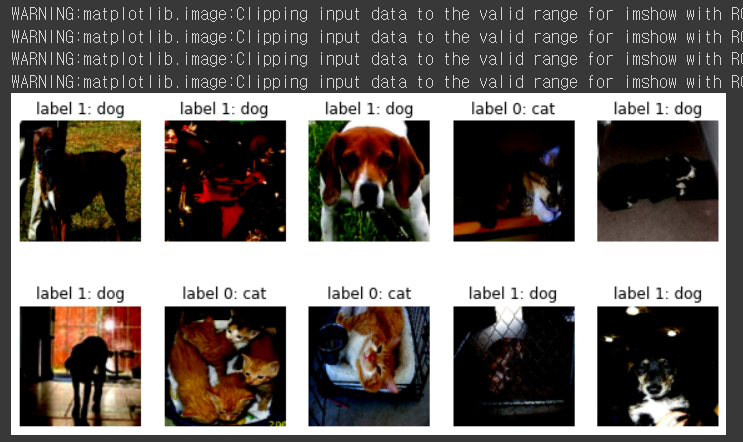
Create Model
데이터 준비가 완료되었으니 딥러닝 모델을 바닥부터 쌓아 봅니다
from tensorflow.keras.models import Sequential
from tensorflow.keras.layers import Dense, Conv2D, MaxPooling2D,Flatten

Model = Sequential([
                    Conv2D(filters=16, kernel_size=3, padding='same', activation='relu', input_shape=(160,160,3)),
                    MaxPooling2D(),
                    Conv2D(filters=32, kernel_size=3, padding='same', activation='relu'),
                    MaxPooling2D(),
                    Conv2D(filters=64, kernel_size=3, padding='same', activation='relu'),
                    MaxPooling2D(),
                    Flatten(),
                    Dense(units=512, activation='relu'),
                    Dense(units=2, activation='softmax')
])
Model.summary()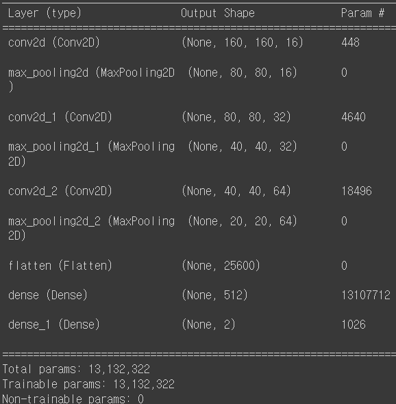
참고 그림으로 간단하게 원리를 살펴봅니다
현재의 이미지들은 결국 최종 1 x 1 x dense 만큼 차원이 줄어들게 됩니다

잘게 잘라진 특성들은 다시 평탄화(flatten) 과정을 거치는데 이를 넘파이로 간단하게 이해하고 넘어가겠습니다
import numpy as np
image = np.array([[1,2],[3,4]])
print(image.shape)
image
#result
(2, 2)
array([[1, 2],
       [3, 4]])

image.flatten()
#result
array([1, 2, 3, 4])
Modify Model
모델의 하이퍼파라미터를 정하고 컴파일 합니다
lr학습비율이며 작게 설정하는 것이 일반적 입니다
로스함수는 크로스 엔트로피이고 모델 성능 측정 지표는 정확도로 판단합니다
learning_rate = 0.0001
Model.compile(optimizer=tf.keras.optimizers.RMSprop(lr=learning_rate),
              loss=tf.keras.losses.sparse_categorical_crossentropy,
              metrics=['accuracy'])
Modify data batch size
모델에 입력할 데이터의 갯수를 정하고 데이터를 섞을 수치도 정합니다
BATCH_SIZE = 32
SHUFFLE_BUFFER_SIZE = 1000
train_batches = train.shuffle(SHUFFLE_BUFFER_SIZE).batch(BATCH_SIZE)
validation_batches = validation.batch(BATCH_SIZE)
test_batches = test.batch(BATCH_SIZE)
배치가 제대로 동작한다면 데이터가 32개씩 묶인 것을 확인할 수 있습니다
for image_batch, label_batch in train_batches.take(1):
    pass

image_batch.shape, label_batch.shape

#result
(TensorShape([32, 160, 160, 3]), TensorShape([32]))
학습 없이 그냥 테스트하면 형편 없는 정확도를 볼 수 있습니다
validation_steps = 20
loss0, accuracy0 = Model.evaluate(validation_batches, steps=validation_steps)
print("initial loss: {:.2f}".format(loss0),"initial accuracy{:.2f}".format(accuracy0),sep="\n")

#result
initial loss: 0.69
initial accuracy0.54
Model Train
생각만큼 만족스러운 결과가 나오지 않습니다
알만한 사람은 알겠지만 요즘 이미지 분류에서 90%는 기본으로 넘어줘야 써먹을만한 시대죠
epoch = 10
history = Model.fit(train_batches,
                    epochs=epoch,
                    validation_data=validation_batches)
Report
acc = history.history['accuracy']
val_acc = history.history['val_accuracy']

loss=history.history['loss']
val_loss=history.history['val_loss']

epochs_range = range(epoch)

plt.figure(figsize=(12, 8))
plt.subplot(1, 2, 1)
plt.plot(epochs_range, acc, label='Training Accuracy')
plt.plot(epochs_range, val_acc, label='Validation Accuracy')
plt.legend()
plt.title('Training and Validation Accuracy')

plt.subplot(1, 2, 2)
plt.plot(epochs_range, loss, label='Training Loss')
plt.plot(epochs_range, val_loss, label='Validation Loss')
plt.legend()
plt.title('Training and Validation Loss')
plt.show()
그림으로 보니 더욱 선명하게 느껴지는 과적합의 향기네요

예측 결과를 통해 어떤 사진이 문제가 있었는지 확인해보기
for image_batch, label_batch in test_batches.take(1):
    images = image_batch
    labels = label_batch
    predictions = Model.predict(image_batch)
    pass

predictions = np.argmax(predictions, axis=1)

plt.figure(figsize=(20,12))

for idx, (image, label, prediction) in enumerate(zip(images, labels, predictions)):
    plt.subplot(4, 8, idx+1)
    image = (image + 1) / 2 # make image positive
    plt.imshow(image)
    correct = label == prediction
    title = f'real:{label} / pred :{prediction}\n {correct}!'
    if not correct:
        plt.title(title, fontdict={'color':'red'})
    else:
        plt.title(title,fontdict={'color':'blue'})
        plt.axis('off')
Pretrained Model
사실 요즘은 바닥부터 만들기보다는 이미 누군가 만들어둔, 그리고 공공연하게
입증된 모델을 사용하는 것이 효율이 좋습니다
공공연하게 입증된 모델이라함은 역시 입상 경력이 있는 모델일테구요
따라서 유서깊은 ILSVRC 대회의 모델을 불러서 사용해보려고 합니다
이때 pretrained model을 불러오더라도 바로 사용하는 것이 아닌
전이 학습의 단계를 거치게 됩니다
전이학습이란
전이학습은 높은 정확도를 비교적 짧은 시간 내에 달성할 수 있기 때문에 컴퓨터 비전 분야에서 유명한 방법론 중 하나입니다 (Rawat & Wang 2017). 전이학습을 이용하면, 이미 학습한 문제와 다른 문제를 풀 때에도, 밑바닥에서부터 모델을 쌓아올리는 대신에 이미 학습되어있는 패턴들을 활용해서 적용시킬 수 있습니다. 이를 샤르트르 식으로 표현하면 거인의 어깨에 서서(standing on the soulder of giants) 학습하는 것이라고 할 수 있겠습니다!
학습을 위해서 Fine Tuning을 할텐데 여기에서는 불러오는 모델의 classifier만 살짝 바꿔줄 예정입니다
어떠한 파인튜닝을 적용해야 좋은지에 대한 조건은 다음의 그림을 참고해주세요

# Load VGG16 model
img_shape = (img_size, img_size, 3)
# load pretrained model
base_model = tf.keras.applications.VGG16(input_shape=img_shape,
                                         include_top=False,
                                         weights='imagenet')
모델 객체인 base_model로 image_batch를 넣으면 model의 입력값에 맞는 batch로 변경됩니다
# how batch size change
feature_batch = base_model(image_batch)
feature_batch.shape
VGG16의 구조


VGG16 - Convolutional Network for Classification and Detection
How does VGG16 neural network achieves 92.7% top-5 test accuracy in ImageNet, which is a dataset of over 14 million images belonging to 1000 classes.
neurohive.io
pretrained model compile
모델의 하이퍼파라미터를 조정하며 컴파일을 합니다
base_learning_rate = 0.0001
model.compile(optimizer=tf.keras.optimizers.RMSprop(learning_rate=base_learning_rate),
              loss=tf.keras.losses.sparse_categorical_crossentropy,
              metrics=['accuracy'])
아직 학습전이라 정확도가 형편없습니다 훈련 후의 값을 보도록 할게요
validation_steps=20
loss0, accuracy0 = model.evaluate(validation_batches, steps = validation_steps)

print("initial loss: {:.2f}".format(loss0))
print("initial accuracy: {:.2f}".format(accuracy0))

#result
loss : 0.93
accuracy : 0.53
이미 수많은 이미지로 학습을 완료한 모델이기 때문에 에포크는 크지 않아도 빠르게 정확도가 올라갑니다
EPOCHS = 5

history = model.fit(train_batches,
                    epochs=EPOCHS,
                    validation_data=validation_batches)
Report
acc = history.history['accuracy']
val_acc = history.history['val_accuracy']

loss = history.history['loss']
val_loss = history.history['val_loss']

plt.figure(figsize=(16, 8))
plt.subplot(1, 2, 1)
plt.plot(acc, label='Training Accuracy')
plt.plot(val_acc, label='Validation Accuracy')
plt.legend(loc='lower right')
plt.ylabel('Accuracy')
plt.ylim([min(plt.ylim()),1])
plt.title('Training and Validation Accuracy')

plt.subplot(1, 2, 2)
plt.plot(loss, label='Training Loss')
plt.plot(val_loss, label='Validation Loss')
plt.legend(loc='upper right')
plt.ylabel('Cross Entropy')
plt.ylim([0,1.0])
plt.title('Training and Validation Loss')
plt.xlabel('epoch')
plt.show()
공인된 모델로 하니 말할 것도 없이 좋은 결과가 나와줍니다
for image_batch, label_batch in test_batches.take(1):
    images = image_batch
    labels = label_batch
    predictions = model.predict(image_batch)
    pass

predictions = np.argmax(predictions, axis=1)

plt.figure(figsize=(20, 12))

for idx, (image, label, prediction) in enumerate(zip(images, labels, predictions)):
    plt.subplot(4, 8, idx+1)
    image = (image + 1) / 2
    plt.imshow(image)
    correct = label == prediction
    title = f'real: {label} / pred :{prediction}\n {correct}!'
    if not correct:
        plt.title(title, fontdict={'color': 'red'})
    else:
        plt.title(title, fontdict={'color': 'blue'})
    plt.axis('off')
모두 맞춰서 파란 글씨네요 정답률을 보겠습니다
count = 0
for image, label, prediction in zip(images, labels, predictions):
    correct = label == prediction
    if correct:
        count = count + 1

print(count / 32 * 100)

# result
100.0
비록 제가 바닥부터 모델을 다진 것은 아니지만 해당 모델을 응용해서 성공적으로 주어진 Task를 수행할 수 있었습니다
이미 입증된 모델을 사용하면 큰 GPU 컴퓨팅 능력도 필요없이 응용해서 만들 수 있기 때문에 효율적이며
동시에 거인의 어깨에 타는 효과를 누릴 수 있었습니다
텐서플로우에서 주어지는 데이터셋과, 모델을 활용해서 더 재밌는 것들을 만들 수 있을 것 같아 기대가 됩니다!
'23년 이전 글 > 모두의연구소 아이펠' 카테고리의 다른 글
| 아이펠 인공지능 교육과정 중간 회고 (0) | 2022.01.14 |
|---|---|
| - 14일차 - 야너두 작사가 될 수 있어 (3) | 2022.01.13 |
| - 12일차 - 너의 얼굴은( Object Detection) (0) | 2022.01.11 |
| -11일차- Everything in Python is Object (0) | 2022.01.10 |
| -10일차- Machine Learning과 Scikit-Learn (0) | 2022.01.07 |